Diffusion Models
Introduction#
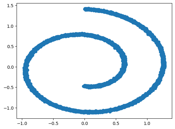
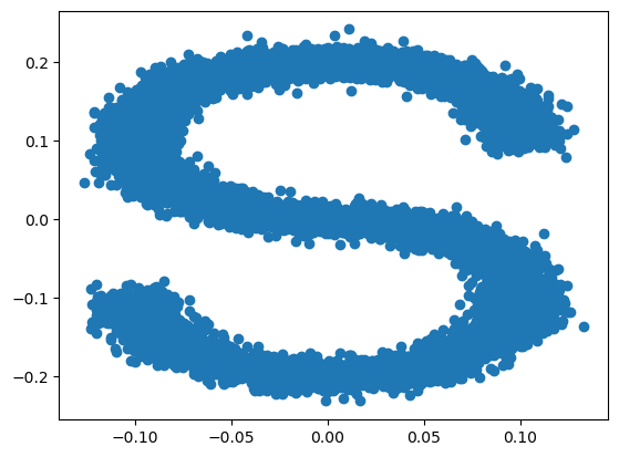
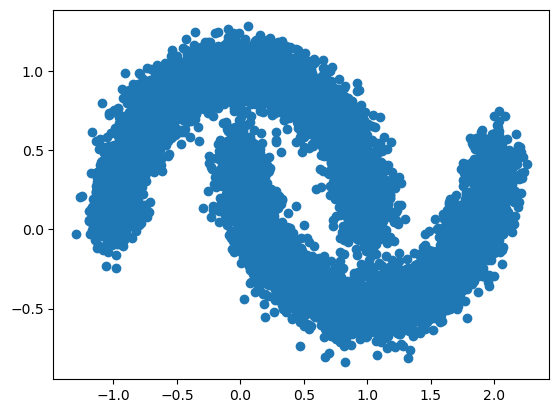
Diffusion probabilistic model (DPM) or just diffusion models are a generative model that has received a lot of attention in the last couple of years in models DALL-E2 and Imagen. In this blog post I will give a short introduction and a minimal implementation of this model. The task we are going to solve is to recover a 2D shape from a random set of points.
The diffusion framework consist of a forward diffusion process were random noise is added to the input until the it has no reassembles to the input. And a reverse process were a neural network learns to undo this process. That is go from a pure noise input to a sample from the target distribution (usually images or audio).

For a compleate derivation of the formulas and some other concepts see this and this posts
import torch
from tqdm.auto import tqdm
import numpy as np
import matplotlib.pyplot as plt
from sklearn.datasets import make_checkerboard, make_circles, make_moons,make_s_curve, make_swiss_roll

device = torch.device("cuda" if torch.cuda.is_available() else "cpu")
# device = torch.device("cpu")

swiss_roll, _ = make_swiss_roll(10**4,noise=0.1)
swiss_roll = swiss_roll[:, [0, 2]]/10.0

s_curve, _= make_s_curve(10**4, noise=0.1)
s_curve = s_curve[:, [0, 2]]/10.0

moons, _ = make_moons(10**4, noise=0.1)

dataset = torch.Tensor(swiss_roll).float().to(device)
print(dataset.shape)

plt.scatter(swiss_roll[:, 0], swiss_roll[:, 1])
plt.show()

plt.scatter(s_curve[:, 0], s_curve[:, 1])
plt.show()

plt.scatter(moons[:, 0], moons[:, 1])
plt.show()

T = 100
torch.Size([10000, 2])


Forward process#
We add Gaussian noise to the input from $t = 0, 1, \cdots, T$ according to the rule:
$$ q(\mathbf{x}_t \vert \mathbf{x}_{t-1}) = \mathcal{N}(\mathbf{x}_t; \sqrt{1-\beta_t}\mathbf{x}_{t-1}, \beta_t\mathbf{I}) $$
in thw last time step ($t=T$) we only have Gaussian noise. The sequence $\beta_t$ is known variance schedule. In general we can afford grater variance in later steps and thus $\beta_0 < \beta_1 \cdots < \beta_T$. This equation says that we sample a noise from a standard gaussian distribution, $\epsilon \sim \mathcal{N}(0, \mathbf{I})$ and then setting $\mathbf{x}_t = \sqrt{1-\beta_t}\mathbf{x}_{t-1} + \sqrt{\beta_t}\epsilon$
def get_betas(T=1000, s=0.0001, e=0.02, type='linear'):
    if type == 'linear':
        return torch.linspace(s, e, T)
    if type == 'sigmoid':
        return torch.sigmoid(torch.linspace(-6, 6, T)) * (e - s) + s
    if type == 'quadratic':
        return torch.linspace(s**0.5, e**0.5, T) ** 2
    else:
        raise NotImplementedError

betas = get_betas(T, type='sigmoid').to(device)
plt.plot(betas.cpu())
plt.show()

Because we are adding gaussian noise at each step there is a nice property that will alow us to sample from any step in the process without having to calculate the previous steps. By defining $\alpha_t = 1 - \beta_t$, $\bar{\alpha}_t = \prod_{s = 0}^T \alpha_s$, and $\mathbf{\epsilon} \sim \mathcal{N}(0, \mathbf{I})$,
$$ \begin{align} \mathbf{x}_t &= \sqrt{1-\beta_t}\mathbf{x}_{t-1} + \sqrt{\beta_t}\mathbf{\epsilon}_t \\ &= \sqrt{\alpha_t}\mathbf{x}_{t-1} + \sqrt{1 - \alpha_t}\mathbf{\epsilon}_t \\ &= \sqrt{\alpha_t\alpha_{t-1}}\mathbf{x}_{t-2} + \sqrt{1 - \alpha_t\alpha_{t-1}}\mathbf{\epsilon}_{t-1} \\ &= \cdots \\ &= \sqrt{\bar{\alpha}_t}\mathbf{x}_0 + \sqrt{1 -\bar{\alpha}_t}\mathbf{\epsilon} \end{align} $$
Where we use the fact that when multipling two Gaussian distributions, $\mathcal{N}(0, \sigma_1^2)$, $\mathcal{N}(0, \sigma_2^2)$, the results distributes $\mathcal{N}(0, \sigma_1^2 + \sigma_2^2)$. With this we can write
$$ q(\mathbf{x}_t | \mathbf{x}_0) = \mathcal{N}(x_t; \sqrt{\bar{\alpha}_t}\mathbf{x}_0, \sqrt{1 -\bar{\alpha}_t}\mathbf{I}) $$
alphas = 1 - betas.to(device)
bar_alpha = torch.cumprod(alphas, dim=0).to(device)
sqrt_bar_alpha = torch.sqrt(bar_alpha)
bar_alpha_prev = torch.nn.functional.pad(bar_alpha[:-1], (1, 0), value=1.0).to(device)
sqrt_minus_one_bar_alpha = torch.sqrt(1 - bar_alpha)
sigma_t = betas * (1 - bar_alpha_prev) / (1 - bar_alpha)

def extract(x, t):
    s = x.shape
    # print(t.device, x.device)
    out = x.gather(-1, t)
    shape = [-1,] + [1]*(len(s))
    return out.reshape(*shape)

def q_sample(x, t, noise=None):
    if noise is None:
        noise = torch.randn_like(x)
    sqrt_bar_alpha_t = extract(sqrt_bar_alpha, t)
    sqrt_minus_one_bar_alpha_t = extract(sqrt_minus_one_bar_alpha, t)
    # print(x.device, sqrt_bar_alpha_t.device, sqrt_minus_one_bar_alpha_t.device, noise.device)
    return sqrt_bar_alpha_t*x + sqrt_minus_one_bar_alpha_t*noise

fig, axs = plt.subplots(1, 10, figsize=(50, 5))
for i, t in enumerate(range(0, T, 10)):
    x_t = q_sample(dataset, torch.tensor([t], device=device)).cpu()
    axs[i].scatter(x_t[:, 0], x_t[:, 1])
    axs[i].set_title(f"t={t}")

Reverse Diffusion#
As mentioned above the idea is to learn the reverse diffusion process, that is given a sample of noise at $\mathbf{x}_T \sim \mathcal{N}(0, \mathcal{I})$ recover the original undistorted data. The quantity $q(\mathbf{x}_{t-1} | \mathbf{x}_t)$ is untractable because it needs knowledge of the underlying distribution. The idea is to train a neural network to approximate this distribution. Notice that for small $\beta_t$ the distribution will also be Gaussian. With some math described in the blog posts mentioned above the network can be viewed as a noise predictor ($\mathbf{\epsilon}_\theta(\mathbf{x}_t, t)$)
$$ \mathbf{\mu}_\theta (\mathbf{x}_t, t) = \frac{1}{\sqrt{\alpha_t}} \left(\mathbf{x}_t - \frac{\beta_t}{\sqrt{1 - \bar{\alpha}_t}}\mathbf{\epsilon}_\theta(\mathbf{x}_t, t)\right) $$
Then a simplified version of the loss is:
$$ L = \vert\vert\mathbf{\epsilon} - \mathbf{\epsilon}_\theta(\sqrt{\bar{\alpha}_t}\mathbf{x}_0 + \sqrt{1 - \bar{\alpha}_t}\mathbf{\epsilon}, t)\vert\vert^2 $$
In summery we have the following algorithms for training and sampling

Model#
The model needs as input the previous sample ($\mathbf{x}_t$) and the current time step $t$ because we use the same network for each step. Here we use a simple learned embeddings and an attention mechanism to condition each layer.
import torch.nn as nn
import torch.nn.functional as F

class ConditionalLinear(nn.Module):
    def __init__(self, num_in, num_out, n_steps):
        super(ConditionalLinear, self).__init__()
        self.num_out = num_out
        self.lin = nn.Linear(num_in, num_out)
        self.embed = nn.Embedding(n_steps, num_out)
        self.embed.weight.data.uniform_()

    def forward(self, x, y):
        out = self.lin(x)
        gamma = self.embed(y)
        out = gamma.view(-1, self.num_out) * out
        return out

class ConditionalModel(nn.Module):
    def __init__(self, n_steps):
        super(ConditionalModel, self).__init__()
        self.lin1 = ConditionalLinear(2, 128, n_steps)
        self.lin2 = ConditionalLinear(128, 128, n_steps)
        self.lin3 = ConditionalLinear(128, 128, n_steps)
        self.lin4 = nn.Linear(128, 2)

    def forward(self, x, y):
        x = F.softplus(self.lin1(x, y))
        x = F.softplus(self.lin2(x, y))
        x = F.softplus(self.lin3(x, y))
        return self.lin4(x)
Training#
There is nothing especial here, just an standard training loop
@torch.no_grad()
def sample():
    x = torch.randn(dataset.shape).to(device)
    xs = [x]
    for t in range(T-1, 0, -1):
        t = torch.tensor([t], device=device)
        at = extract(alphas, t)
        at1 = extract(sqrt_minus_one_bar_alpha, t)
        z = torch.randn(dataset.shape, device=device) if t > 1 else 0.0
        x = 1/torch.sqrt(at) * (x - (1 - at)/at1 * model(x, t)) + extract(sigma_t, t)*z
        xs.append(x)
    return xs

def plot_xs(xs):
    fig, axs = plt.subplots(1, 10, figsize=(50, 5))
    for i, t in enumerate(range(0, T, 10)):
        x_t = xs[i*10].cpu()
        axs[i].scatter(x_t[:, 0], x_t[:, 1])
        axs[i].set_title(f"t={t}")
    plt.show()
model = ConditionalModel(T).to(device)
optimizer = torch.optim.Adam(model.parameters(), lr=1e-3)
dataset = dataset.to(device)
loss_fn = torch.nn.MSELoss()
batch_size = 128

for epoch in tqdm(range(1000)):
    permutation = torch.randperm(dataset.shape[0])
    for i in range(0, dataset.shape[0], batch_size):
        indices = permutation[i:i+batch_size]
        batch = dataset[indices]
        t = torch.randint(0, T, (batch.shape[0],), device=device).long()
        noise = torch.randn_like(batch)
        xt = q_sample(batch, t, noise)

        loss = loss_fn(noise, model(xt, t))
        loss.backward()

        torch.nn.utils.clip_grad_norm_(model.parameters(), 1.)
        optimizer.step()

    if epoch % 100 == 0:
        print(loss)
        xs = sample()
        plot_xs(xs)
tensor(0.6853, device='cuda:0', grad_fn=<MseLossBackward0>)

tensor(0.5163, device='cuda:0', grad_fn=<MseLossBackward0>)

tensor(0.5630, device='cuda:0', grad_fn=<MseLossBackward0>)

tensor(0.8198, device='cuda:0', grad_fn=<MseLossBackward0>)

tensor(0.7627, device='cuda:0', grad_fn=<MseLossBackward0>)

tensor(0.7034, device='cuda:0', grad_fn=<MseLossBackward0>)

tensor(0.8251, device='cuda:0', grad_fn=<MseLossBackward0>)

tensor(0.4305, device='cuda:0', grad_fn=<MseLossBackward0>)

tensor(0.5074, device='cuda:0', grad_fn=<MseLossBackward0>)

tensor(0.3056, device='cuda:0', grad_fn=<MseLossBackward0>)

xs = sample()
plot_xs(xs)

Conclusion#
Diffusion models are currently in the state of the art in varius generation tasks surpassing GANs and VAE in some metrics. Here I presented a simple implementation of the main elements of a diffusion model. One of the disadvantages of this class of models is in the sampling speed because there are $T$ network evaluations.
