Physics informed neural networks

April 13, 2023

Introduction

Physics informed neural networks (PINNs) is a framework for solving PDEs first introduced in 1998 by Lagaris et al. and later in 2019 where reintroduced to the DL community by Raissi et al. The main idea is to train an artificial neural network that follow physics given by a PDE.

Sample problem

In this article I will be using the logistic equation known to model population growth as a one dimensional example problem. This equation requiers three parameters, the growth rate $r$ and the carrying capacity $K$, and the initial population $u(0)$. The equation is:

$$ \frac{d}{dt} u - r u (1 - \frac{u}{K}) = 0 $$

Because we will need it later the left hand side of the equation will be called $f(u, t) = \frac{d}{dt} u - r u (1 - \frac{u}{K})$. Using standar methods this equation can be solved analytically as

$$ u(t) = u(0)K\frac{e^{rt}}{K + u(0)(e^{rt} - 1)} $$

In many practical situations this is not posible and one has to use numerical approximations. In this article will set $u(0)=0.01$, $r=10.0$ and $K=2.0$

import numpy as np
import matplotlib.pyplot as plt

domain = [0.0, 1.0]
r = 10.0
K = 2.0
u0 = 0.1
x_eval = np.linspace(domain[0], domain[1], 100)

def logistic(x):
    return u0 * K * np.exp(r*x) / (K + (u0*np.exp(r * x) - 1))

plt.plot(x_eval, logistic(x_eval))

The framework proposes to train a neural network that will approximate the analytical solution $u(t)\approx NN_\theta(t)$. The network is supervised by two losses. A boundary loss that forces the network to satisfy the initial and boundary condition given in the set of points ${t_i}$.

$$ MSE_u = \frac{1}{N}\sum_{i=1}^{N} (u(t_i) - NN_\theta(t_i))^2 $$

And a interior loss that enforces the structure imposed by the equation for a set of collocation points ${t_j}$

$$ MSE_f = \frac{1}{N}\sum_{j=1}^{N} f(NN_\theta(t_j), t_j)^2 $$

Thus the final loss is

$$ \mathcal{L}(\theta) = MSE_u + MSE_f $$

Is important to note that we will need to take derivatives of the network’s output with respect to it’s input. This is no problem thanks to the build in automatic differentiation of deep learning frameworks.

Now that we know the problem lets define an artificial neural network in pytorch that will serve as our approximation to the solution to our problem.

import torch
import torch.nn as nn

device = torch.device("cuda" if torch.cuda.is_available() else "cpu")

class ANN(nn.Module):
    def __init__(self, num_hidden_layers, num_hidden_dims, act=nn.Tanh()):
        super().__init__()
        self.layer_in = nn.Linear(1, num_hidden_dims)
        self.layer_out = nn.Linear(num_hidden_dims, 1)
        self.hidden_layers = nn.ModuleList(
            [nn.Linear(num_hidden_dims, num_hidden_dims) for _ in range(num_hidden_layers - 1)])

        self.act = act

    def forward(self, x):
        x = self.layer_in(x)
        x = self.act(x)
        for l in self.hidden_layers:
            x = l(x)
            x = self.act(x)
        x = self.layer_out(x)
        return x

Model fitting

The first application deals with the case the solution is known only at the boundary (u(0)) and the parameters are also know. This can method can be used as an alternative to classical numerical methods for solving PDEs such as finite elements and Runka-Tuka. This is generally known as the forward problem.

The following functions calculate the value of the function, it's derivative and the loss function.

Here we use the parametrization $u(0) + x NN_\theta(x)$ for the solution. Notice how this parametrization automatically satisfies the boundary conditions and the only the interior loss is necessary.

def f(nn, x):
    return u0 + x*nn(x)

def df(nn, x, order=1):
    df_value = f(nn, x)
    for _ in range(order):
        df_value = torch.autograd.grad(
            df_value,
            x,
            grad_outputs=torch.ones_like(x),
            create_graph=True,
            retain_graph=True,
        )[0]

    return df_value

def compute_loss(nn, x):
    u = f(nn, x)
    intirior_loss = (df(nn, x) - r * u * (1 - u/K)).pow(2).mean()
    return intirior_loss

This function is a standard training loop in pytorch. Note that we are using L-BFGS as an optimizer. This second order method converges more quickly than standard first order methods

def train_model(nn, loss_fn, lr=0.01, epochs=1000):
    loss_evolution = []

    nn.to(device)
    # optimizer = torch.optim.RMSprop(nn.parameters(), lr=lr)
    optimizer = torch.optim.LBFGS(nn.parameters(), lr=lr)
    def closure():
        optimizer.zero_grad()
        loss = loss_fn(nn)
        loss.backward()
        return loss

    for epoch in range(epochs):

        loss = loss_fn(nn)
        optimizer.zero_grad()
        loss.backward()
        optimizer.step(closure)
        # optimizer.step()

        if epoch % 100 == 0:
            print(f"Epoch: {epoch} - Loss: {float(loss):g}")

        loss_evolution.append(loss.cpu().detach().numpy())
    nn.cpu()
    return nn, np.array(loss_evolution)

We create a set of collation points and train the network

from functools import partial

x = torch.linspace(domain[0], domain[1], steps=10, requires_grad=True)
x = x.reshape(x.shape[0], 1) # colacation points

NN = ANN(2, 20)

loss_fn = partial(compute_loss, x=x.to(device))
nn_trained, loss_evolution = train_model(
        NN, loss_fn=loss_fn, lr=0.1, epochs=500
    )

    Epoch: 0 - Loss: 2.20393
    Epoch: 100 - Loss: 8.05022e-07
    Epoch: 200 - Loss: 6.88934e-07
    Epoch: 300 - Loss: 6.88934e-07
    Epoch: 400 - Loss: 6.88934e-07

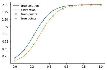
Next let’s plot the solution and compare it to the ground truth.

x_eval = torch.linspace(domain[0], domain[1], steps=100).reshape(-1, 1)
x = x.cpu()

f_eval = f(nn_trained, x_eval).detach().numpy()
f_train = f(nn_trained, x).detach().numpy()
f_true = logistic(x.detach().numpy())

x = x.detach().numpy()

plt.plot(x_eval, logistic(x_eval), label="true solution")
plt.plot(x_eval, f_eval, '--', label="estimation")
plt.plot(x, f_train, 'x', label="train points")
plt.plot(x, f_true, '.', label="true points")
plt.legend()
plt.show()

print("Error:", np.mean((f_eval - logistic(x_eval.detach().numpy())) ** 2))

plt.semilogy(loss_evolution)
plt.show()

    Error: 0.029134285

We can see the network quickly learns to replicate the true solution form some combinations of $r$, $K$ and $u(0)$. For some values it fails to learn the function.

Finding parameters

A second approach to PINNs is when the solution is know at the boundary and some other set of points, but the parameters ($r$ and $K$) of the equation are unknown. This setting is sometimes referred as the inverse problem. The loss function is the same as before only that the set ${t_i}$ includes points were the solution is known.

def f(nn, x):
    return nn(x)

def df(nn, x, order=1):
    df_value = f(nn, x)
    for _ in range(order):
        df_value = torch.autograd.grad(
            df_value,
            x,
            grad_outputs=torch.ones_like(x),
            create_graph=True,
            retain_graph=True,
        )[0]

    return df_value

def compute_loss(nn, x, u_star, x_c):
    u = f(nn, x_c)
    intirior_loss = (df(nn, x_c) - (r_est * u * (1 - u/K_est))).pow(2).mean()

    boundary_loss = (f(nn, x) - u_star).pow(2).mean()
    # print(u, intirior_loss, boundary_loss)
    return intirior_loss + boundary_loss

The main difference here is that we added the parameters r_est and K_est to the network so they are updated along with the weights. Let’s train and see the results

from functools import partial

x_c = torch.linspace(domain[0], domain[1], steps=10, requires_grad=True) # colacation points
x_c = x_c.reshape(x.shape[0], 1)

x = torch.tensor(np.random.uniform(domain[0], domain[1], size=10).astype("float32"), requires_grad=True)
x = x.reshape(x.shape[0], 1)
u_star = torch.tensor(logistic(x.detach().numpy()), requires_grad=True)

r_est = torch.tensor([1.0], requires_grad=True).to(device)
K_est = torch.tensor([1.0], requires_grad=True).to(device)

r_est = torch.nn.Parameter(r_est)
K_est = torch.nn.Parameter(K_est)

NN = ANN(4, 128).to(device)
NN.register_parameter('r', r_est)
NN.register_parameter('K', K_est)

loss_fn = partial(compute_loss, x=x.to(device), u_star=u_star.to(device), x_c=x_c.to(device))
nn_trained, loss_evolution = train_model(
        NN, loss_fn=loss_fn, lr=0.1, epochs=500
    )

    Epoch: 0 - Loss: 2.34788
    Epoch: 100 - Loss: 2.59089e-06
    Epoch: 200 - Loss: 2.59089e-06
    Epoch: 300 - Loss: 2.59089e-06
    Epoch: 400 - Loss: 2.59089e-06

x_eval = torch.linspace(domain[0], domain[1], steps=100).reshape(-1, 1)
x = x.cpu()

f_eval = f(nn_trained, x_eval).detach().numpy()
f_train = f(nn_trained, x).detach().numpy()
f_true = logistic(x.detach().numpy())

x_train = x.detach().numpy()

plt.plot(x_eval, logistic(x_eval), label="true solution")
plt.plot(x_eval, f_eval, '--', label="estimation")
plt.plot(x_train, f_train, 'x', label="train points")
plt.plot(x_train, f_true, '.', label="true points")
plt.legend()
plt.show()

print("Error:", np.mean((f_eval - logistic(x_eval.detach().numpy())) ** 2))
print("r_est:", r_est.detach().numpy()[0], "r real", r)
print("K_est:", K_est.detach().numpy()[0], "K real", K)

plt.semilogy(loss_evolution)
plt.show()

:::

    Error: 2.9455983e-08
    r_est: 10.001771 r real 10.0
    K_est: 1.9999409 K real 2.0

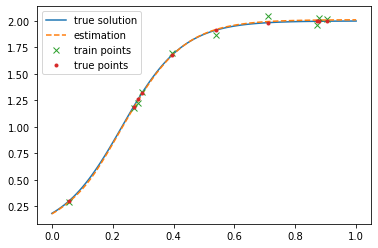
We observe that the network is capable of both adjusting to the unknown equation and find the parameters.

With noisy data

In real life there is always some amount of uncertainty in the measured data. We can model this by disturbing the points with random noise.

from functools import partial
x_c = torch.linspace(domain[0], domain[1], steps=10, requires_grad=True) # colacation points
x_c = x_c.reshape(x.shape[0], 1)

x = torch.tensor(np.random.uniform(domain[0], domain[1], size=10).astype("float32"), requires_grad=True)
x = x.reshape(x.shape[0], 1)
u_star = torch.tensor(logistic(x.detach().numpy()) + np.random.normal(scale=0.05, size=x.shape), requires_grad=True)


r_est = torch.tensor([1.0], requires_grad=True).to(device)
K_est = torch.tensor([1.0], requires_grad=True).to(device)

r_est = torch.nn.Parameter(r_est)
K_est = torch.nn.Parameter(K_est)

NN = ANN(4, 128).to(device)
NN.register_parameter('r', r_est)
NN.register_parameter('K', K_est)

loss_fn = partial(compute_loss, x=x.to(device), u_star=u_star.to(device), x_c=x_c.to(device))
nn_trained, loss_evolution = train_model(
        NN, loss_fn=loss_fn, lr=0.1, epochs=500
    )

    Epoch: 0 - Loss: 2.77947
    Epoch: 100 - Loss: 0.000890755
    Epoch: 200 - Loss: 0.000890755
    Epoch: 300 - Loss: 0.000890755
    Epoch: 400 - Loss: 0.000890755

x_eval = torch.linspace(domain[0], domain[1], steps=100).reshape(-1, 1)
x = x.cpu()

f_eval = f(nn_trained, x_eval).detach().numpy()
f_train = f(nn_trained, x).detach().numpy()
f_true = logistic(x.detach().numpy())

x_train = x.detach().numpy()

plt.plot(x_eval, logistic(x_eval), label="true solution")
plt.plot(x_eval, f_eval, '--', label="estimation")
plt.plot(x_train, u_star.detach().numpy(), 'x', label="train points")
plt.plot(x_train, f_true, '.', label="true points")
plt.legend()
plt.show()

print("Error:", np.mean((f_eval - logistic(x_eval.detach().numpy())) ** 2))
print("r_est:", r_est.detach().numpy()[0], "r real", r)
print("K_est:", K_est.detach().numpy()[0], "K real", K)

plt.semilogy(loss_evolution)
plt.show()

    Error: 0.0001071914
    r_est: 9.946944 r real 10.0
    K_est: 2.011487 K real 2.0

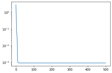
We can see that the network finds a balance between fitting the data and obeying the equation.

Sanity check, are we just fitting the data?

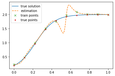
As proof that we are doing something by adding the physics lets train a network with only a loss on the known points.

def f(nn, x):
    return nn(x)

def df(nn, x, order=1):
    df_value = f(nn, x)
    for _ in range(order):
        df_value = torch.autograd.grad(
            df_value,
            x,
            grad_outputs=torch.ones_like(x),
            create_graph=True,
            retain_graph=True,
        )[0]

    return df_value

def compute_loss(nn, x, u_star):
    u = f(nn, x)
    boundary_loss = (u - u_star).pow(2).mean()
    return boundary_loss

from functools import partial


x = torch.linspace(domain[0], domain[1], steps=10, requires_grad=True)
x = x.reshape(x.shape[0], 1) # colacation points
u_star = torch.tensor(logistic(x.detach().numpy()) + np.random.normal(scale=0.05, size=x.shape), requires_grad=True)


NN = ANN(4, 128).to(device)

loss_fn = partial(compute_loss, x=x.to(device), u_star=u_star.to(device))
nn_trained, loss_evolution = train_model(
        NN, loss_fn=loss_fn, lr=0.1, epochs=500
    )

    Epoch: 0 - Loss: 2.50134
    Epoch: 100 - Loss: 7.18925e-10
    Epoch: 200 - Loss: 7.18925e-10
    Epoch: 300 - Loss: 7.18925e-10
    Epoch: 400 - Loss: 7.18925e-10

x_eval = torch.linspace(domain[0], domain[1], steps=100).reshape(-1, 1)
x = x.cpu()

f_eval = f(nn_trained, x_eval).detach().numpy()
f_train = f(nn_trained, x).detach().numpy()
f_true = logistic(x.detach().numpy())

x_train = x.detach().numpy()

plt.plot(x_eval, logistic(x_eval), label="true solution")
plt.plot(x_eval, f_eval, '--', label="estimation")
plt.plot(x_train, u_star.detach().numpy(), 'x', label="train points")
plt.plot(x_train, f_true, '.', label="true points")
plt.legend()
plt.show()

print("Error:", np.mean((f_eval - logistic(x_eval.detach().numpy())) ** 2))

plt.semilogy(loss_evolution)
plt.show()

    Error: 0.023793427

For the outside data the model does a weird nonlinear interpolation of the data and does not predict a logistic equation. Also the network is not robust against noise the predictions pass throw the noisy samples and not close to the real data.

Train with data on a single region

Now let’s consider a more challenging situation. In this case the data is kwon only at one region of the domain.

def f(nn, x):
    return nn(x)

def df(nn, x, order=1):
    df_value = f(nn, x)
    for _ in range(order):
        df_value = torch.autograd.grad(
            df_value,
            x,
            grad_outputs=torch.ones_like(x),
            create_graph=True,
            retain_graph=True,
        )[0]

    return df_value

def compute_loss(nn, x, u_star, x_c):
    u = f(nn, x_c)
    intirior_loss = (df(nn, x_c) - (r_est * u * (1 - u/K_est))).pow(2).mean()

    boundary_loss = (f(nn, x) - u_star).pow(2).mean()
    # print(u, intirior_loss, boundary_loss)
    return intirior_loss + boundary_loss

from functools import partial
x_c = torch.linspace(domain[0], domain[1], steps=10, requires_grad=True) # colacation points
x_c = x_c.reshape(x.shape[0], 1)

x = torch.tensor(np.random.uniform(domain[0], domain[1]/10, size=10).astype("float32"), requires_grad=True)
x = x.reshape(x.shape[0], 1)
u_star = torch.tensor(logistic(x.detach().numpy()) + np.random.normal(scale=0.05, size=x.shape), requires_grad=True)


r_est = torch.tensor([1.0], requires_grad=True).to(device)
K_est = torch.tensor([1.0], requires_grad=True).to(device)

r_est = torch.nn.Parameter(r_est)
K_est = torch.nn.Parameter(K_est)

NN = ANN(4, 128).to(device)
NN.register_parameter('r', r_est)
NN.register_parameter('K', K_est)

loss_fn = partial(compute_loss, x=x.to(device), u_star=u_star.to(device), x_c=x_c.to(device))
nn_trained, loss_evolution = train_model(
        NN, loss_fn=loss_fn, lr=0.1, epochs=500
    )

    Epoch: 0 - Loss: 0.079713
    Epoch: 100 - Loss: 0.00346369
    Epoch: 200 - Loss: 0.00346369
    Epoch: 300 - Loss: 0.00346369
    Epoch: 400 - Loss: 0.00346369

x_eval = torch.linspace(domain[0], domain[1], steps=100).reshape(-1, 1)
x = x.cpu()

f_eval = f(nn_trained, x_eval).detach().numpy()
f_train = f(nn_trained, x).detach().numpy()
f_true = logistic(x.detach().numpy())

x_train = x.detach().numpy()

plt.plot(x_eval, logistic(x_eval), label="true solution")
plt.plot(x_eval, f_eval, '--', label="estimation")
plt.plot(x_train, u_star.detach().numpy(), 'x', label="train points")
plt.plot(x_train, f_true, '.', label="true points")
plt.legend()
plt.show()

print("Error:", np.mean((f_eval - logistic(x_eval.detach().numpy())) ** 2))
print("r_est:", r_est.detach().numpy()[0], "r real", r)
print("K_est:", K_est.detach().numpy()[0], "K real", K)

plt.semilogy(loss_evolution)
plt.show()

    Error: 3.9343088
    r_est: 8.156542 r real 10.0
    K_est: 5.087321 K real 2.0

We can se the model converges correctly to a logistic function. If only a narrow portion of the data is given it may fail to predict accurately the parameters.

Conclusions

PINNs are a powerfull tool for solving PDEs, in both the forward and inverse problems.